
Acknowledgements
I would like to thank Dr. Gwynfor Richards for giving me this area to pursue for my seminar topic, and for helping me when I was totally stuck during the coding portion of it. Id also like to thank Scott Schaefer for his help through his subdivision website. Finally Id like to thank Shauna for supporting me in all of this (especially when I wouldnt keep quiet when something did not work correctly).
Notes
This revision of this document has changed slightly since its original creation. It has been combined into one single document, instead of multiple documents, and formatted accordingly.
All of the source code for this project is available for download on my personal website at http://www.granite.mb.ca/~joey/. I would encourage those who are interested in this paper and this particular area of computer graphics to download and try them. As stated in the project review, the code was developed under Microsoft Visual Studio .NET. As such, the project files are in that format as well.
Abstract
The purpose of this project was to develop a better understanding of subdivision surfaces and their use in computer graphics. By the end of this project, I was able to implement a few simple subdivision schemes, and apply them to meshes of varying complexity. This paper goes over some of the theory behind subdivision surfaces, and includes some information on how to implement them.
1. Introduction
I am working in a particular field of three-dimensional graphics referred to as subdivision surfaces. It involves the smoothing of concave meshes into smoothed approximations of themselves. This area was originally developed for three dimensions by Doo and Sabin, and Catmull and Clark, during the 1970s.
Before subdivision surfaces were used, b-spline patches had to be used to create a smooth surface. Instead of creating a surface composed of smooth curves, we create one using a coarse base mesh, and recursively subdivide its polygons and perturb the vertices of the polygons until we approximate a smooth surface.
This is used primarily in the fields of animation, games, and the scanning of three-dimensional objects. Pixar began using this technology and incorporating it into their RenderMan software when they began running into the limitations of NURBS (non-rational uniform b-splines, a form of b-splines used to create smooth surfaces).
Im doing this research to better my understanding of subdivision surfaces, and some of the methods used to develop and create them. Out of this research, I have been able to develop a few programs using C++ and OpenGL using the glut toolkit, that allow me to subdivide triangular and quadrilateral meshes of varying complexity.
Though this is a relatively young field, there have been quite a large number of papers written about it in recent years, and such algorithms have been included in 3D modeling and rendering packages such as Maya and Blender. The algorithms and schemes behind subdivision are generally straightforward and easy to understand.
Ill begin by outlining some theory behind subdivision surfaces, and follow by describing some algorithms and schemes used to create them. From there, Ill describe where and how this particular area of computer graphics is used, and finally describe what I did to implement my own subdivision surface schemes, and any problems that I faced while implementing them.
2. Literature Review
2.1 What Subdivision Surfaces Are
A subdivision surface is a polygonal mesh that has been subdivided and smoothed. It is a mesh that has had every polygon sliced into two or more polygons, and then has each vertex moved to a calculated location. Though this is a simple description, there are many schemes and algorithms available to subdivide any given mesh, in numerous ways.
Since subdivision surfaces are algorithmic, they can also be defined recursively to find a smoothness level that is acceptable, by allowing the designer of the mesh to choose a particular level to subdivide to.
2.2 Why Use Subdivision Surfaces
2.2.1 NURBS and B-Splines
Usually when an artist using a 3D modeling package wants to create a perfectly smooth surface, they must use a NURBS (non-rational uniform b-spline surface) patch. This is a grid of control points joined by smooth curves in three dimensions that approximates a smooth surface. While this works, the main problem with these patches is that if two are to be placed next to each other, the number of vertices along their width and their height has to be equal on both patches, otherwise discontinuities may become visible in the surface of the final mesh [7]. This gives the artist another thing to worry about during creation time. It also limits the artist to creating something that is composed entirely of quadrilaterals, as opposed to using a strictly triangular based mesh.
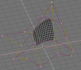 Figure 1. A 3 by 3 NURBS patch in the Blender modeling environment. |
2.2.2 Speed
In the case where an artist will be doing a lot of work on a mesh with a large polygon count, they can save considerable time by employing a coarse base mesh, subdividing and editing it from that point forwards. Working with a high polygon-count mesh interactively is usually a high-demand operation on either the processor or video hardware. By reducing the amount of polygonal data that the artist is working with, we can reduce the load put onto the artists system.
2.3 Where Subdivision Surfaces Are Used Now
2.3.1 3D Modeling and Rendering
Subdivision surfaces are being included in modeling and rendering packages because of their ease of use, and the freedom they allow the artist. They are even beginning to become one of the modeling primitives [4], which would see them being included in almost every modeling package available.
Skeletal animation incorporates itself nicely into subdivision surfaces, since the mesh is just dependent on the bones of the underlying skeleton. Once a basic mockup of a character mesh is created, and the animation details are worked out, all that the artist should have to do is subdivide their mesh. From there, everything will be in complete control of the skeletal animation system [6].
2.3.2 3D Scanning
When an object is scanned into a computer using a 3D scanner, there are often artifacts (i.e. small bulges or bumps where there were not any on the original object) or missing areas that the scanner just could not pick up. Subdivision surfaces could easily take the existing data brought in from the scanner, and interpolate where missing data should be placed, and remove any artifacts from the surface of the mesh.
2.3.3 Game Development
With the processing and graphics power of personal computers and gaming consoles ever-increasing, it would make sense to start subdividing character models depending on the current performance any machine is experiencing. If the frame rate of the game is running higher than normal, the game engine could allow the character meshes to increase in complexity, without loss of speed in the game. The converse is also true; if the frame rate is starting to run low, the game engine could reduce the complexity of the character meshes on screen to increase the frame rate of the game.
Level of detail control also comes into play. If a character mesh is far off into the background, the game engine could draw it using 100 to 200 polygons, rather than 2,000. Complex meshes could be saved for close-ups, or low action scenes where the frame rate of the game does not make a difference.
Finally, most character meshes currently use texture mapping to represent clothing, markings, and other visual information on the character. Since most 3D video hardware is designed for generating hundreds upon thousands of polygons, texture mapping could be removed altogether. Instead of mapping an image of the letter "M" on Mario, the artist could paint it on in the model editor. A coloured polygon is less taxing to draw than a textured one, so this could in theory free up the video hardware to draw more coloured polygons, resulting in higher quality meshes. (See [1] for more information on this area).
2.4 What Makes a Good Subdivision Surface Scheme
2.4.1 Continuity
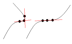 Figure 2. Two curves exhibiting C0 continuity on the left, and C1 continuity on the right. |
The whole purpose of a subdivision surface scheme is to achieve a continuous smooth surface. Smoothness is described in terms of continuity, where continuity refers to the degree of the derivatives. A surface which is C0 has derivatives of degree 0 where two edges meet at a vertex, which would include sharp edges with no apparent smoothness. A surface has C1 continuity if the first derivatives of each edge meeting at a vertex are equal; this type of continuity removes most sharp edges and seams over a surface. Some schemes will even create areas which are C2 continuous (i.e. the second derivatives are equal for each edge meeting up at a vertex).
2.4.2 Approximating and Interpolating Schemes
Though smoothness is a main concern, the next major concern is whether the scheme is interpolating or approximating. An approximating scheme will for the most part stay inside its own control net (the control net is the low polygon count mesh that is the starting point for subdivision), and just approach the surface of the control net. Approximating meshes will always stay within the confines that are set for it (for most cases, there are a few exceptions).
An interpolating scheme keeps all of the vertices from the control net on the final limit surface. New vertices are added between the existing vertices, which allow the final form of the mesh to appear closer to the control net. Unfortunately, because of the interpolative nature of these meshes, small bumps or undulations in the surface are removed from the final mesh. These types of meshes are better used for meshes which are C1 continuous where there is not going to be a lot of variation over the surface of the mesh itself.
2.4.3 Uniformity
Uniformity refers to how edges are subdivided. In a uniform scheme, all edges are subdivided the same way, no matter what their location or valence is. A non-uniform scheme would subdivide different edges different ways. For example, and edge that is on a boundary of a mesh would have vertices added to it in a different way than an edge that was elsewhere in the mesh.
Related to uniformity is whether or not the scheme is stationary. A stationary mesh uses the same set of rules at each step of subdivision. A non-stationary mesh uses different steps at different points of subdivision. For instance, in one of the programs, a triangular mesh is subdivided into quadrilaterals for the first subdivision step; from that point forward, all subdivision steps are applied to a quadrilateral mesh.
2.4.4 Shape and Extraordinary Vertices
The shape of a mesh refers to what kinds of polygons are used to build a mesh. As mentioned in the last section, I used triangular and quadrilateral meshes for my subdivision programs, which are built out of triangles and quadrilaterals respectively. Though these programs just operate strictly on polygons of a particular number of edges and vertices (i.e. strictly triangles, quadrilaterals, pentagons, etc.), it is possible to have a mesh composed of many different polygons. The problem with this is that it generates what is called an extraordinary vertex.
The number of edges that meet at a vertex is called the vertexs valence (or its degree). When a triangular mesh is split up, most of the vertices are of degree six. Similarly, when we split up a quadrilateral mesh, most of the vertices are of degree four; these are referred to as ordinary vertices. An extraordinary vertex is one that is not of the standard degree in the given mesh. So for a triangular mesh, an extraordinary vertex could of degree three, four, or five.
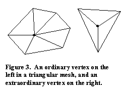 The
problem with extraordinary vertices is that they do not smooth as nicely
as ordinary vertices. This will usually make the final surface appear to
have thin spikes "poking" out at various places around the mesh. These anomalies
can be fixed using correction terms that take into account the valence of
the particular vertex being looked at.
2.4.5 Evaluation Masks
An evaluation mask is used to determine what vertices to use when calculating a vertexs position. Sometimes called a stencil, it can vary in shape and size, and is sometimes used after linear subdivision is done, or after the main subdivision step is done, and applied only to ordinary or extraordinary vertices. The butterfly scheme uses evaluation masks, and is explained in further detail below.
2.4.6 Support and Locality
When a surface is subdivided, the algorithm usually iterates over the polygons or vertices in the mesh itself. The neighbouring vertices of a particular vertex are used to determine how to perturb the vertex to achieve smoothing. This is known as local support. Without this local support, the artist who is creating the mesh will have to go back and make slight alterations in other areas of the mesh. Almost all schemes have local support.
2.5 Overview of a Few Subdivision Schemes
There are numerous subdivision schemes that differ in the meshes that they operate on, and how they act upon those meshes. Most to all of them generate surfaces with C1 continuity, and deal with the problems of extraordinary vertices in their own way. There are multiple ways of implementing some of these schemes, so just one example is given for each.
 2.5.1
Linear/Polyhedral Subdivision
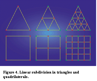
This scheme just subdivides the existing polygons in the mesh into more polygons. It does not provide any more than C0 continuity over the surface of the mesh. It is a uniform, stationary scheme with local support. It is also interpolating since it does not move any of the original vertices within the mesh. For triangular meshes, it is designed so that it splits a single triangle into four using the midpoints of the original triangle. Quadrilateral subdivision requires us to create a new vertex in the centre of the quadrilateral itself to create four new quadrilaterals for the mesh (see Figure 3).
Although this mesh does not produce a smooth surface, it is sometimes used for two-pass schemes where we first need to produce new vertices in the mesh before any smoothing is done.
2.5.2 Loop Subdivision
Developed by Charles Loop for his Masters Thesis, this scheme operates only on triangular meshes. It was created to be able to approximate a smooth surface without having to rely on B-splines or NURBS patches, but the mathematics are still based on those mathematics.
This is an interpolating mesh so it is C1 continuous, so we actually have a smooth surface at the end of subdivision. Like linear subdivision, it is also approximating, and uniform.
2.5.3 Doo-Sabin Subdivision
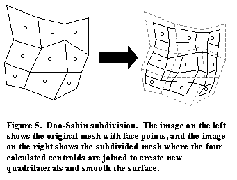 This
is where most research began into subdivision, and this was developed Daniel
Doo, and Michael Sabin. It was actually a refinement on what George Chaikin
did to approximate quadratic uniform b-splines [3].
Using the centroid of a quadrilateral, and the midpoints of each edge, four centroids can be calculated. They used this information to create four points within the each quadrilateral. These four points could be used to create new quadrilaterals, which would be connected to their neighbours. This approximation gives the mesh the appearance that large chunks are being cut off the corners. If this is continued, we can approximate a smooth surface (see Figure 4).
Though it is meant for quadrilateral meshes, it can be extended so that it is possible to smooth meshes of arbitrary polygons.
This scheme is approximating and has C1 continuity [8]; it is also uniform since the rules dont change from one iteration to the next.
2.5.4 Catmull-Clark Subdivision
This particular scheme is probably the most researched, and the most used in the realm of high-end graphical rendering. This scheme is what Pixar used to create their smooth surfaces in "Geris Game", and is also available as a smoothing scheme in the open source 3D modeling tool, Blender. It was first developed in the 1970s by Ed Catmull, and Jim Clark, and is based on the mathematics behind bicubic uniform B-Spline surfaces, and is based off similar work to that of Doo and Sabin.
This is one scheme that depends on the polyhedral scheme to subdivide the surface first before any vertices are perturbed (see Figure 3). It is meant to operate on quadrilateral meshes by adding a vertex to the center of every quadrilateral (called a face point), and then joining each midpoint on each surrounding edge to the face point itself. From there the surface is smoothed as the average of Q, 2R, S(n-3), where:
Q The average of the new face points of all faces adjacent to the original face point,
R The average of all the midpoints of all original edges incident on the original vertex point,
S The original vertex point, and
n The degree of the original vertex point.
This scheme is meant to operate on quadrilateral meshes, but can actually be slightly modified to operate on a mesh of arbitrary polygons. As mentioned earlier, it is possible to generate quadrilaterals from any given polygon. Though this does introduce an extraordinary vertex into the mesh, Catmull-Clark has a correction term to prevent any problems from popping up. This scheme is approximating since the original vertices in the mesh are moved. Uniformity is dependant on whether the mesh being subdivided consists strictly of quadrilaterals. After doing the first subdivision step, the rules are strictly uniform for each successive step.
There has been even more done for Catmull-Clark surfaces, one of the main features being the ability to support sharp creases in the surface. With these, the designer of the mesh picks edges they wish to stay sharp, and to what degree they should remain sharp. During the subdivision process, the edges are basically ignored and left as sharp or semi-sharp creases.
Like Doo-Sabin, this scheme is C1 continuous [8], and is also uniform (provided it is running on a quadrilateral mesh). Also, even though this is an approximating mesh, it is possible with some meshes to have the final surface extend outside of its control net (for more on this, see the Project Review).
2.5.5 Butterfly and Modified Butterfly Subdivision
The butterfly scheme is one that depends on using a stencil to calculate the smoothness of the surface. That is what the term butterfly describes in this context, the shape of the stencil used to determine which vertices are used to perturb the current vertex. It also uses a tension parameter to determine how close to the limit surface the final mesh approaches.
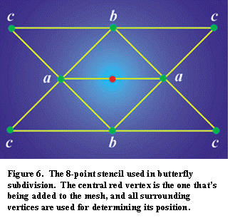 The
coefficients in Figure 5 refer to how much they affect the current vertexs
position. They break down to the following:
a: 1/2
b: 1/8 + 2w
c: -1/16 w
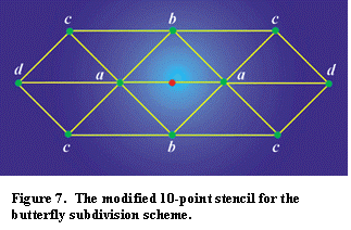
The parameter w is the tension parameter for this scheme. If w equals 0, c is left as -1/16, which just linearly interpolates the mesh; this leaves behind undesired sharp areas on the final surface. One solution theorized at one point was to use a 10-point stencil with a fourth parameter, d, which is just equal to w.
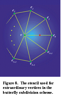
Unfortunately, this scheme had a similar problem in that it could lead the current vertex to being twice as far from where it started out from. Eventually a stencil was created by Zorin, Schröder, and Sweldens as an extension to the butterfly scheme to make the surface C1 everywhere [6]. The vertexs new position is now determined by this stencil, and a new set of rules, where both ends of the current edge were taken into account. This new stencil was applied only to extraordinary vertices; ordinary vertices continued using the ten point stencil (see Figure 6).
The weights used for this new stencil are:
N = 3: (v: ¾, e0: 5/12, e1: -1/12, e2:
-1/12)
N = 4: (v: ¾, e0: 3/8, e1: 0, e2:
-1/8, e3: 0)
N ≥ 5: (v: ¾, ej:(0.25 + cos(2πj/N)
+ 0.5 * cos(4 πj/N))/N)
2.5.6 Other Methods
As mentioned above, there are multiple ways of achieving the same smoothed surface given any particular scheme. It is possible to create fractal subdivision surfaces. Although it seems to be used less for character meshes and single objects, there seems to be a lot of use for it in terrain generators. Since a fractal looks the same zoomed in as it does when zoomed out, a large amount of detail can be generated very quickly with very little code needing to be written.
The methods used for the demonstration programs are based on Loop and Catmull-Clark subdivision surfaces, but are not implemented strictly by them. They both use a similar algorithm for linearly subdividing the mesh and then doing vertex averaging to calculate the new positions of the vertices. Theses schemes do approximate Loop and Catmull-Clark very well, and are approximating, C1 continuous, uniform schemes. They are based on the subdivision schemes described by Joe Warren and Scott Schaefer in "A Factored Approach to Subdivision". These are described in much more detail in the Project Review.
2.6 Related Areas
2.6.1 Mesh Simplification
If subdivision surfaces are used for adding more detail and curvature to a model, mesh simplification could be described as the complete opposite. The whole purpose of mesh simplification is to remove excess data from our mesh. It is later subdivided to approximate our original mesh. The whole reason for doing this is to cut down on the amount of information needed for permanent mesh storage. Further detail goes beyond the scope of this paper, so please refer to [4] for more information.
3. Project Review
3.1 Overview
I set out to create a few simple programs to subdivide meshes of arbitrary complexity, and I was able to do that by projects end. I chose to use the methods described by Scott Schaefer in his paper "A Factored Approach to Subdivision", and have gotten some great results from it. I chose to use his methods mainly because of their simplicity to understand and implement.
3.2 Using the Programs
Once any of the programs have started, the following key commands can be used to manipulate them. Please note that since the number of polygons is typically increased by a factor of four for each step of subdivision that the programs may pause for processing time before resuming control to the user.
X, Y, Z: Increment the speed at which the mesh rotates around the x, y, and z axes respectively.
S: Stop the mesh from moving.
B: Enable/Disable wireframe control net.
Space: Switch to wireframe view.
F4/F5: Move the camera up and down respectively (along the y-axis).
Up/Down: Move the camera in and out (along the z-axis).
+/-: Increase and decrease level of subdivision accordingly.
F1: Enable/Disable fullscreen view.
Esc: Quit program.
3. 3 Libraries and Data Structures Used
All of the coding for these programs was done using Microsoft Visual C++.NET in a Win32 environment. The graphics portion was handled by GLUT (OpenGL Utility Toolkit), rather than Microsofts own DirectX. I chose the OpenGL library for its ease of use in setting up, and its platform agnostic design, in case I decided to port some of my code to another platform (i.e. Linux, Mac OS X, Irix, etc.). Finally, I used the STLs vector classes to reduce any possible memory leaks in the programs themselves, to prevent any major hits in performance.
For handling the data of the meshes themselves, I created a set of classes to handle all of the geometry that would need to be stored for each mesh. They are as follows:
Vertex: Stores x, y, z coordinate information, as well as RGB colour information. I also have data reserved for normal vectors for smooth shading, but they are currently unused as I felt that it would be a large performance hit for each iteration of subdivision we did. Also, smooth shading would make it difficult to notice the change between each level of subdivision.
Triangle: Stores three indices into an array of vertices that represents a triangle. These indices are ordered so that the triangle is drawn counter-clockwise. It also stores the normal vector to the plane that the triangle is in for lighting purposes.
Quadrilateral: Similar to Triangle except it contains four indices to represent a quadrilateral.
TriangularMesh: Contains an array of vertices, and an array of triangles, which is fed into this object through a file read function. Also keeps track of the current number of vertices, edges and triangles in the mesh, and also calculates the degree of each vertex, and the normal of each triangle in the mesh.
QuadrilateralMesh: Similar to TriangularMesh except that it operates on quadrilaterals.
TriangularMeshRenderer & QuadrilateralMeshRenderer: Classes designed to take the meshes and draw them to the screen using OpenGL. It should be noted that these two classes are designed to be platform independent, and could easily be ported to another system with little to no changes for compilation.
Hash: What should have been a two-key hash table is actually implemented as a 2 dimensional matrix. This is used during linear subdivision to determine if two vertices are adjacent to each other. The object-oriented structure behind this class should make it very easy to implement an actual two-key hash table without any effect the programs themselves.
PolySub: A set of static classes to subdivide the triangles in a TriangularMesh object to smaller triangles, and to perturb the vertices to approximate Loop subdivision.
QuadSplit: Similar to PolySub, but instead acts on QuadrilateralMesh objects, and approximates Catmull-Clark subdivision.
TriQuad: Like PolySub and QuadSplit, but this class is designed to linearly split triangles into quadrilaterals.
3.4 Data Files
The mesh files themselves are loaded into the program using text files that contain vertex, polygon, and colour data. They consist of a version number, the number of vertices and polygons in the mesh as well as what polygons are used, vertex and vertex colour data, and finally indices into the vertices themselves.
3.5 Algorithm Overview
The only thing that differs between the programs that I have written is what particular set of algorithms I have used to subdivide the particular mesh that has been loaded into the program. All of these algorithms subdivide the mesh linearly since they generate four polygons for each polygon they split (three for third program), and thus the number of polygons increases linearly as we subdivide the meshes.
3.5.1 Program #1: Triangular Subdivision
This program first linearly subdivides the mesh that is fed into it. This is done by passing over each triangle in the mesh, and splitting the triangle into four smaller triangles.
Given a vertex vi, we can take the vertex vi + 1 and see if it is in our hash table. If there is nothing stored at that location, we store the index of the new vertex that is being added to that location. If the same two vertices appear again later on, we can just pull the index of the new vertex right out of the hash table. The colour data for the midpoints is also calculated by taking the colour of vertices vi and vi+1 and dividing by two.
Once this is done, we can create four new triangles, by using the vertices of the original triangle, and all of the midpoints that we calculated in the last step.
T0: {v0, m0, m2}
T1: {v1, m1, m0}
T2: {v2, m2, m1}
T3: {m0, m1, m2}
Linear subdivision is completed after each triangle has been split up this way. Finally the vertex degrees are calculated, as well as the number of edges counted and stored in the mesh object. The next step is to call the perturb() function and smooth the mesh.
This is accomplished by first creating an array of vertices for the new positions that need to be calculated for the perturbed vertices; all of these are initialized to (0, 0, 0). We then iterate over the each triangle in the mesh and calculate its centroid. We then add the centroid coordinates and our original vertex coordinates to our array of new vertex positions. Next, we divide each vertex by its degree. If it is not an extraordinary vertex, we have to include a weighting factor to prevent any sharp spikes from appearing in the mesh. The weighting factor for our mesh is:
w(n) = 5/3 8/3(3/8 + 1/4cos(2π/n))2
This weight is applied thusly, where vi is our current vertex from our mesh, and Ni is the new vertex:
vi + w(n)Ni vi
Finally, we set colour data for the vertex by copying the colour information from the original vertex from the mesh. For dealing with extraordinary vertices, we just assign the value of the new position that we calculated earlier. At this point we re-calculate the normal vectors for each triangle for lighting purposes.
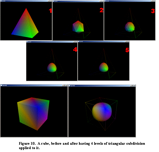 |
3.5.2 Program #2: Quadrilateral Subdivision
A lot of the techniques from the previous section apply to the quadrilateral subdivision case. Again, we subdivide the mesh linearly, turning each quadrilateral we come across into four quadrilaterals. We again generate a new vertex for each midpoint between each pair of vertices we come across, but we also generate a face point in the center of each quadrilateral. Once these vertices have been calculated, we create four quadrilaterals according the following rules. Again, colour for the new vertices is calculates during this step as well.
Q0: {m0, v1, m1, c}
Q1: {m1, v2, m2, c}
Q2: {m2, v3, m3, c}
Q3: {m3, v0, m0, c}
We now call the perturb() function to smooth out the mesh. The method described above for triangular subdivision follows very closely to what we do for quadrilateral meshes. We create a new array of vertices with each element initialized to (0, 0, 0), and then add the original vertex data along with the calculated centroid vertex data. From there we divide each vertex by its associated valence, and for extraordinary vertices, we apply a different weighting factor (different from the one used for Loop subdivision):
w(n) = 4 / n.
Finally, the number of edges, and a normal vectors for each polygon are calculated.
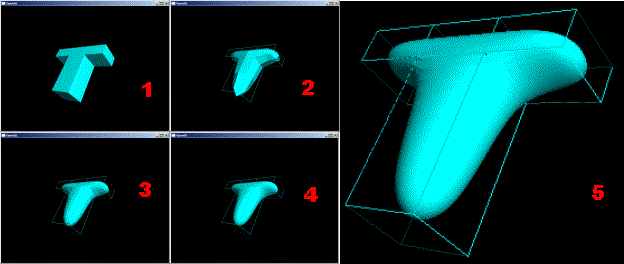 Figure 11. A mesh subdivided with the Catmull-Clark approximating scheme. The last image shows that the final surface extends outside of its base control net. |
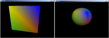

3.5.3 Program #3: Quadrilateral Subdivision With Triangles
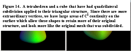
 With the above programs, I just used triangular subdivision
methods for triangle-based meshes, and quadrilateral subdivision for quadrilateral-based
meshes. The final example I wrote, I decided to try using Catmull-Clark
style subdivision on a non-quadrilateral based mesh. The algorithm is pretty
generalized, so it was not too difficult to design it for a triangle-based
mesh. Although it is not usually recommended to use Catmull-Clark on a mesh
that is not composed of quadrilaterals, I found that although it could only
give C1 continuity over extraordinary vertices, this did allow
my meshes to keep more of their structure as opposed to having them condense
to a spherical/elliptical shape with no real sense of what the original mesh
looked like.
 |
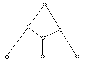
Again, it follows the same system of first subdividing the mesh linearly, followed by a perturbing the vertices to make them appear to smooth the mesh. The only difference in this version of the algorithm is that for linear subdivision, we break each triangle into three quadrilaterals instead of four triangles. This is done by calculating the centroid to the triangle, and joining each midpoint of the triangle to this point. From there, we create four triangles based on the rules used during Catmull-Clark subdivision. Perturbing the vertices is handled the same way.

3.7 Improvements
It has been often said that a programmer never knows when his program is finally complete, and no program is ever truly bug free. This is certainly true of my programs as well, but as far as I am concerned all the major bugs are removed. This just leaves extra features to be added.
As I mentioned in the description of the data structures, I included room for normal vector for each vertex. It would be nice to have a function that went through and calculated these for each subdivision step to enable smooth shading, but again, it is a performance hit that I see for the time being as unnecessary. Also, storing data for texture coordinates and textures as well to see how they would have acted under subdivision itself would be interesting to note.
A binary data structure would be a bit faster, and would be even better than having to calculate all the points on paper, enter them manually into a text editor, and re-compile the source to see how it looked and how it acted under subdivision. It would be a lot more convenient to use a program like Blender and use its open data structure to load data into the programs.
Any other work that I would end up doing beyond this would be strictly redesigning the programs and their data structures. I left most if not all of the vertex data as public, for ease of typing. It did not appeal to me to write separate GetX(), GetY(), GetZ(), SetX(), SetY(), and SetZ() methods for the coordinate data. It would also have been unpleasant to do the same for the colour, and normal vector data as well. The last major design change to possibly make would be to separate the OpenGL rendering code further away from the core of the program, so any other graphics API could be used (i.e. DirectX, software rendering, etc.).
3.8 Polygon Count Table
Included is a count of the number of polygons at each step of subdivision for the meshes shown in this document.
Program #1
Polygon Count of Triangular Meshes Using Triangular Subdivision |
|||||
Mesh |
0 |
1 |
2 |
3 |
4 |
Pyramid |
6 |
24 |
96 |
384 |
1536 |
Cube |
12 |
48 |
192 |
768 |
3072 |
Dragon |
609 |
2436 |
9744 |
38976 |
155904 |
Program #2
Polygon Count of Quadrilateral Meshes Using Quadrilateral Subdivision |
|||||
Mesh |
0 |
1 |
2 |
3 |
4 |
Cube |
6 |
24 |
96 |
384 |
1536 |
BigT |
18 |
72 |
288 |
1152 |
4608 |
Program #3
Polygon Count of Triangular Meshes After Applying Quadrilateral Subdivision |
|||||
Mesh |
0 |
1 |
2 |
3 |
4 |
Pyramid |
6 |
18 |
72 |
288 |
1152 |
Cube |
12 |
36 |
144 |
576 |
2304 |
Dragon |
609 |
1827 |
7308 |
29232 |
116928 |
4. Conclusion
Since I started looking into this area in September, Ive been able to better understand subdivision surfaces, some of the algorithms and schemes behind them, where theyre being used, and what they are being used for. Ive also been able to write my own programs that demonstrate these ideas, and even come up with one that keeps the final subdivided mesh closer to the original mesh we started with.
I have found that once the data structures are properly setup, a scheme can be set up quickly to subdivide any mesh. I have also found that there is a lot of processing power required at higher levels of subdivision because of the large amount of information that are generated from this process. Though this isnt a problem for non-real-time rendering software, real-time rendering software (i.e. those in games) would need a lot of power in terms of doing the subdividing of meshes on the fly, and even optimized algorithms.
5. References
[1] Brickhill, "GDC 2002: Incredibly Dense Meshes". Gamasutra, April 10, 2002. http://www.gamasutra.com/features/20020410/brickhill_01.htm
[2] Joy, "Doo-Sabin Surfaces". On-Line Geometric Modeling Notes, November 28, 2000. http://graphics.cs.ucdavis.edu/CAGDNotes/Doo-Sabin/Doo-Sabin.html
[3] Joy, "Chaikins Algorithms for Curves". On-Line Geometric Modeling Notes, November 28, 2000. http://graphics.cs.ucdavis.edu/CAGDNotes/Chaikins-Algorithm/Chaikins-Algorithm.html
[4] Lee, "Building Your Own Subdivision Surfaces". Gamasutra, September 8, 2000. http://www.gamasutra.com/features/20000908/lee_01.htm
[5] Schaefer, Warren, "A Factored Approach to Subdivision". Rice University, 2003. http://www.cs.rice.edu/~sschaefe/research/tutorial.pdf
[6] Sharp, "Subdivision Surface Theory". Gamasutra, April 11, 2000. http://www.gamasutra.com/features/20000411/sharp_01.htm
[7] Sharp, "Implementing Subdivision Surface Theory". Gamasutra, April 25, 2000. http://www.gamasutra.com/features/20000425/sharp.htm
[8] Zorin, "A Method For Analysis of C1-Continuity of Subdivision Surfaces". NYU Media Research Laboratory. http://mrl.nyu.edu/publications/method-analysis/method.pdf
Images
All images created by Joseph Baumgartner unless otherwise noted.
Figures 4, 6, 7, 8 taken from "Subdivision Surface Theory", by Brian Sharp, April 11, 2000.
Geri from "Geris Game", http://www.noemalab.com/sections/specials/tetcm/animazione_digitale/toy_story_2/images/vecchio.jpg
Meshes
All meshes were created by Joseph Baumgartner unless otherwise noted.
Dragon Mesh, Downloaded from the home page of Dr. Chandrajit Bajaj, http://www.cs.utexas.edu/users/bajaj/graphics23/cs354/project3/polyhedra/dragon.off
 Subdivision Surfaces